How to Fit Text in Excel: Easy Tips for Perfect Cell Alignment

Struggling to make your Excel sheets look neat and professional? You’re not alone.

When text spills out of cells or gets cut off, it can mess up your entire layout and make your data hard to read. But what if you could fix this in just a few simple steps? You’ll discover easy, effective ways to fit text perfectly inside your Excel cells.

Whether you want to save space or make your spreadsheets clearer, these tips will help you take control and impress anyone who sees your work. Ready to master your Excel text? Let’s dive in.

Credit: office-watch.com

Adjusting Column Width

Adjusting column width in Excel helps display your text clearly and neatly. It prevents text from being cut off or hidden behind other cells. Proper column width makes your spreadsheet easy to read and professional.

Excel offers quick ways to change column width to fit your text perfectly. You can use automatic or manual methods based on your needs. Both options are simple and effective for organizing your data.

Autofit Feature

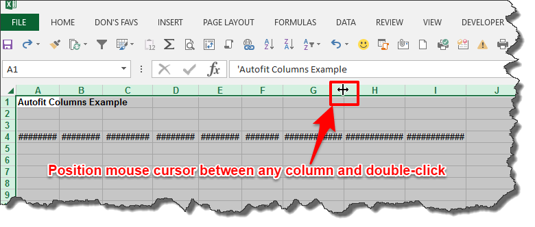
The AutoFit feature adjusts column width to fit the longest text in the column. Double-click the right edge of the column header. Excel expands the column exactly to the text size.

This feature saves time and effort. It works for single or multiple columns at once. Select the columns, then double-click any selected column edge. The columns resize automatically.

Manual Width Adjustment

You can also set the column width manually. Click the column header to select it. Hover over the right edge of the column until the cursor changes.

Drag the edge left or right to resize the column. Stop when the text fits well. You can also right-click the column header, choose “Column Width,” and enter a number.

This method gives precise control over the column size. Use it for custom spacing or design needs.

Credit: www.exceldemy.com

Using Wrap Text

Using Wrap Text in Excel helps you manage long strings of text within a cell without changing the column width. It keeps your spreadsheet tidy and easy to read by displaying all content clearly inside the cell borders. This feature is especially useful when dealing with descriptions, comments, or any multi-line text entries.

Enabling Wrap Text

To enable Wrap Text, first select the cell or range of cells where you want the text to fit better. Then, look for the “Wrap Text” button on the Home tab in the ribbon. Clicking this button will automatically adjust the cell height to show all lines of text inside the cell without overflowing.

You can also enable Wrap Text by right-clicking a cell, choosing “Format Cells,” and then checking the “Wrap Text” box under the Alignment tab. This method gives you more control if you want to apply it to multiple cells at once.

Benefits For Multi-line Text

Wrap Text makes reading and editing easier by breaking long text into multiple lines within the same cell. You avoid the hassle of widening columns excessively, which can disrupt the layout of your spreadsheet. It keeps your data compact and visually accessible.

Imagine you’re listing product details or customer feedback. Without Wrap Text, these entries can become truncated or force you to scroll horizontally. Enabling Wrap Text ensures you see everything at a glance, saving time and reducing errors when reviewing your data.

Have you noticed how much more efficient your workflow becomes when you don’t have to keep adjusting column widths? Wrap Text is one of those small features that can make a big difference in daily spreadsheet management.

Merging Cells

Merging cells in Excel helps manage text that does not fit in a single cell. It combines two or more cells into one larger cell. This technique is useful for titles, labels, or any content that needs more space. It improves the look of your spreadsheet and makes data clearer.

When To Merge Cells

Use merging to create a single header across multiple columns. It works well for center-aligning titles above data. Avoid merging if you need to sort or filter data. Merging is best for formatting, not for organizing raw data. Use it to highlight important sections or group information visually.

How To Merge Properly

• Select the cells you want to merge.
• Go to the Home tab on the Excel ribbon.
• Click the “Merge & Center” button.
• Choose the merge option: Merge & Center, Merge Across, or Merge Cells.
• Check that your text fits well inside the new merged cell.

Remember, merging cells can remove data from all but the upper-left cell. Always save your work before merging. Use merging only when it improves readability without harming data structure.

Changing Row Height

Adjusting row height in Excel is key to making sure your text fits perfectly within cells. Changing row height can improve readability and presentation without distorting your entire worksheet. Whether you want Excel to handle it automatically or prefer to set a specific height, understanding these options will help you control the look of your data.

Automatic Row Height

Excel can automatically adjust the height of rows to fit the content inside cells. This feature is especially useful when you have wrapped text or multiple lines in a cell. To activate it, simply double-click the boundary below the row number on the left side.

Automatic row height saves you from guessing the perfect size. It adapts instantly as you edit or add new information. Have you ever noticed how some rows stay too tight or too loose? This option often fixes that without extra effort.

Custom Row Height Settings

If you want more control, you can set a custom row height. Right-click the row number and select “Row Height.” Then enter the exact number you want. This is great when you need uniform rows or want to match specific design requirements.

Choosing a custom height helps when automatic resizing doesn’t give the look you want. For example, you might want rows taller to improve spacing or shorter to fit more rows on one screen. Have you tried adjusting row height to fit a printed report better? Custom settings can make all the difference. Learn More...

Aligning Text Within Cells

Aligning text within Excel cells improves data clarity and presentation. Proper alignment helps readers scan and understand your content easily. Excel offers several horizontal and vertical alignment options to customize text placement inside each cell. Adjusting alignment creates a tidy and professional look in your spreadsheets.

Horizontal Alignment Options

Horizontal alignment controls text placement from left to right within a cell. Excel has these main horizontal alignment choices:

• Left Align:Text aligns to the left edge of the cell. This is the default for text entries.
• Center Align:Text centers horizontally, balancing space on both sides.
• Right Align:Text aligns to the right edge, common for numbers or dates.
• Justify:Text stretches to fill the entire cell width, spacing words evenly.
• Fill:Text repeats to fill the cell width, useful for patterns or codes.

Select cells, then choose alignment options from the Home tab on the Ribbon for quick adjustments.

Vertical Alignment Options

Vertical alignment adjusts text placement from top to bottom inside a cell. Excel provides three key vertical alignments:

• Top Align:Text sits at the top edge of the cell.
• Middle Align:Text centers vertically between the top and bottom edges.
• Bottom Align:Text rests at the bottom edge, often used for numbers.

Use vertical alignment to improve readability, especially in taller cells or merged cells. Combine horizontal and vertical alignment for optimal text positioning.

Using Shrink To Fit

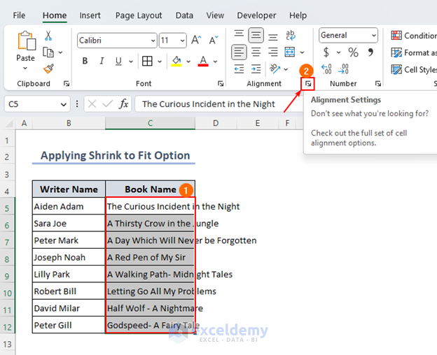
Using Shrink to Fit in Excel helps text fit inside a cell without changing the cell size. It reduces the font size to make the text visible within the cell borders. This feature keeps your spreadsheet neat and easy to read.

Activating Shrink To Fit

To activate Shrink to Fit, select the cell or cells with the text you want to resize. Right-click and choose “Format Cells.” Go to the “Alignment” tab. Check the box labeled “Shrink to Fit.” Click “OK” to apply the change.

The text will automatically reduce in size to fit the cell width. The original font style remains, only the size changes.

When To Use This Feature

Shrink to Fit is useful when you want to keep cell size consistent. It works well for cells with long text that should not wrap or overflow. Use it to maintain clean rows and columns.

It is not ideal for very long text or when font size must stay readable. In such cases, other options like wrapping text or adjusting column width might work better.

Formatting Tips For Better Readability

Proper formatting makes Excel data easier to read and understand. Adjusting font and cell design improves clarity. Small changes help viewers focus on key information.

Font Size And Style

Choose a font size that is clear and not too small. A size between 10 and 12 points works well for most spreadsheets. Use simple fonts like Arial or Calibri for better legibility.

Bold important headers to separate them from regular data. Avoid fancy fonts that distract or look messy. Keep font colors dark on a light background for best contrast.

Cell Padding And Borders

Increase cell padding to add space around text inside cells. This avoids crowding and makes the content easier to scan. Use the “Format Cells” option to add padding.

Apply borders around cells to separate data visually. Thin lines work best to keep the look clean. Use different border styles to highlight totals or important sections.

Credit: medium.com

Frequently Asked Questions

How Do I Wrap Text In Excel?

To wrap text in Excel, select the cell, then go to the “Home” tab. Click “Wrap Text” in the alignment group. This adjusts the cell height to fit the text within. You can also manually adjust the row height by dragging the row boundary.

Can I Resize Cells To Fit Text?

Yes, you can resize cells to fit text. Select the cells, then hover over the column boundary until you see a double arrow. Drag to adjust the width. Alternatively, use “Format” under the “Home” tab and select “AutoFit Column Width.

“

What Is The Shortcut For Fitting Text In Excel?

To quickly fit text, use the shortcut Alt + H + O + I. This auto-adjusts column width based on the longest text in the column. It ensures all text is visible without manual adjustments.

How Do I Use Autofit For Text?

Use AutoFit by selecting cells and then double-clicking the column boundary. This automatically adjusts column width to fit the longest text. Alternatively, use “Format” in the “Home” tab and choose “AutoFit Column Width. “

Conclusion

Fitting text in Excel cells keeps your data clear and tidy. You can adjust column width, row height, or use wrap text easily. These simple steps save time and make spreadsheets look neat. Practice these tips to handle Excel better every day.

Clean, organized sheets help you work faster and avoid mistakes. Try these methods next time you use Excel. It makes a big difference.